Before the Dashboard Knows: Detecting Real-Time Trends in CX Conversations

On the morning of a DHS system outage, the event didn't surface first in one of the airline's ops dashboards or a Slack channel. It surfaced in calls. 

Before internal intelligence had registered anything, travelers were already phoning in about the same failure, checkpoints, and delays faster than any system could update. The airline's contact center knew what was happening hours before the business did.

Real-Time Trends is the system we built to close that gap. It listens to live conversation streams, surfaces emerging topics fast, and presents them as ranked, named headlines with a tracked lifecycle. 

Think of it like a live news feed of what customers are actually telling you right now. 

It does two things existing systems can't. 

1. It catches the unknown unknowns: phishing scams, an unexpected weather event, an app outage, issues that no predefined category would track or that would get buried in something more general. 
2. It quantifies the magnitude of the events you already know about. A geopolitical flashpoint or a new piece of legislation might already be on your radar, but Real-Time Trends surfaces how it's actually landing with customers right now, how many calls it's driving, what the sentiment is, and what solutions people are asking for.

Here is what that looks like to our customers: a live, ranked feed of what is actually moving right now, named, scored, and refreshed throughout the day.

In this post, we’ll walk through how exactly the system works.

The Challenge: Real-time Signal Detection at Scale

The data that makes this useful is also the data that makes it hard.

Contact center traffic is high volume but low per-event signal — a single conversation rarely tells you anything; trends emerge across hundreds. On top sit two qualitatively different challenges. 

1. Linguistic noise — transcription errors, brand-name quirks, plurals, paraphrases, multilingual surface forms — we mostly accept, with downstream clustering closing the most visible gaps. 
2. Temporal drift — the predictable, repeating fluctuations in call volume based on when it is (e.g., morning vs. evening, weekday vs. weekend) — we can subtract: the baseline window is filterable to comparable times of day and days of week (opt-in per customer), so the comparison is against history that looks like now.

Every design decision sits on the same fundamental tradeoff: freshness versus accuracy. Push detection latency to seconds and per-bucket counts are too small to be statistically meaningful — the system fires on noise. Wait a day for stable counts and the value of "real time" disappears. The sweet spot for response/detection time for typical contact center volume is around 30 minutes.

Design Principles

Three commitments shaped the system before any code was written.

Near real-time, not true real-time. The smallest time window in which most customers produce statistically stable counts is on the order of 20 minutes. Targeting lower latency would force the system to detect noise. We accept the 20-minute floor and design around it. The original product target was "refresh every one to two hours"; tightening to 20 minutes still leaves the math intact at typical contact center volume.

Precompute aggressively. Don't query on the fly. Detection runs as a scheduled offline pipeline. The serving API reads precomputed trend records, never recomputes them at request time. This bounds query cost regardless of UI traffic and lets us iterate on the detection algorithm without touching the API surface. The cost is a fixed-latency staleness floor; the benefit is operational stability.

Optimize for recall, filter noise downstream. A real-time trends system that fires too easily becomes wallpaper; one that fires too late becomes irrelevant. We bias toward recall — a missed outage hurts customers far more than a noisy candidate that gets filtered later — and rely on downstream layers (clustering, the LLM noise filter) to keep the surfaced list clean. Every failure mode is biased toward fail-open: if the naming model errors, the trend keeps its phrase as a label. If the noise filter errors, candidates pass through. Silently dropping a real spike is worse than surfacing a noisy one.

What This System Is Not Designed to Solve

To maintain a clear focus on the primary goals of our real-time trends system, the following problems, while interesting, are deliberately excluded from its scope at this time:

• No filter-scoped trends. Trends are computed globally per use case. "Trends inside long calls only" or "trends for new-agent conversations" is a different system.
• No in-product editing of detected key phrases. If a customer wants to track a specific phrase from a detected trend on an ongoing basis, they pin it as a keyword subcategory in Dashboard Builder, which already does curated metric tracking well. Real-Time Trends hands off to Dashboard Builder rather than competing with it.
• No negative-direction trends. Only upward spikes are surfaced. Down-trends (such as a known issue resolving or a campaign cooling) are interesting but a separate product question.

System Architecture

The pipeline has four layers. Each runs independently and can be replaced without rewiring the others.

Ingestion runs on its own cadence; detection runs on its own. They communicate through the analytical store, never directly. Either can be paused, backfilled, or replayed in isolation.

Efficient Signal Extraction From Text

The substrate of the entire system is the n-gram keyphrase — a contiguous run of one to five tokens drawn from normalized conversation text.

The extraction step Unicode-normalizes the text, segments sentences with a multilingual sentence breaker, tokenizes, strips stopwords, and emits every 1- through 5-gram. Multi-word phrases are token-sorted so that "refund request" and "request refund" collapse to the same phrase identifier. So a single message like "i would like a refund for my order" yields candidate phrases such as refund, order, and refund order — no stopwords, canonical form.

Two tradeoffs governed this layer: 

1. Precision over coverage. Literal n-grams are auditable. When a trend fires, the system can point to the exact phrase and the exact conversations that contained it. That property is hard to get from embedding-clustered topics, and it matters for customer trust: trends that cannot be explained are trends that cannot be acted on. The price is that we miss paraphrases and idioms; a downstream LLM clustering step closes the most visible gaps.

2. Cost over fidelity. N-gram extraction is essentially free per message. Embedding every message at ingestion would multiply storage and compute by orders of magnitude. The system spends its richer-representation budget on the small subset of phrases that actually survive into the trending set.

Extraction runs in a small Rust crate exposed to Python through PyO3. The library leans on a few well-trodden building blocks — ICU4X for Unicode normalization and multilingual word and sentence segmentation, Rayon for parallel iteration across messages and conversations, MurmurHash3 to assign each canonicalized phrase a stable 64-bit identifier — and the result is fast enough that ingestion is almost never the bottleneck, even at the highest customer volumes. 

Python is the right language for everything around extraction — gRPC, ClickHouse inserts, workflow orchestration — but customized text processing in a tight per-token loop (canonicalization, sliding n-gram windows, hash-keyed counters) is the shape of code where CPython falls down twice: interpreter overhead on every operation, and the GIL preventing a single process from using more than one CPU core. Rust here is doing real work: extracting 1- through 5-grams from tens of thousands of conversations in seconds, with deterministic output across languages and scripts.

Time-series Aggregation at Scale

The output of aggregation is a per-phrase time series: for each customer, each use case, each 20-minute bucket, how many conversations contained that phrase.

Why 20-minute buckets? It is the smallest window where typical contact-center volume produces stable per-phrase counts, and the largest that still meets the freshness target. Smaller buckets amplify Poisson-like noise; larger buckets dilute spikes and also cut storage, since row count scales inversely with bucket size. We tested both directions.

Aggregation is necessary because the cardinality of distinct n-grams across a multi-month history is in the millions, with a long-tail distribution where the vast majority appear only once or twice. Aggregating into a fixed time grid lets a single short query scan the full historical baseline for thousands of candidate phrases at once, which is what the detection algorithm needs.

Storage is tiered, and we lean heavily on ClickHouse to do the work. Its AggregatingMergeTree engine paired with materialized-view-as-insert-trigger semantics means pre-aggregation happens at write time, in the database itself — no separate batch job to operate. 

An incoming-counts table holds raw per-batch writes with short retention, each row carrying a Map(ngram_id → count) so a single insert records thousands of phrases at once. An aggregated-stats table holds rolled-up counts at the fixed 20-minute grid, populated by a materialized view that deduplicates source rows, expands the maps into per-phrase rows, and merges partial sum states lazily in the background. Column codecs optimized for time-series workloads (Delta + ZSTD for timestamps, T64 + ZSTD for integer counts) reduce the aggregated-stats footprint and improve scan efficiency; partition-level TTL clauses expire old data automatically. A separate cold tier mirrors the aggregated-stats table at a much longer TTL — materialized counts rather than aggregate states — and serves backfill and long-history queries that fall outside aggregated-stats retention.

For per-phrase text lookup ("what surface forms did this n-gram appear as last week?"), the system uses ClickHouse's topKWeighted aggregate state — a probabilistic sketch in the HyperLogLog family — to keep only the top-K most frequent renderings of each phrase per week. The result is a compact, mergeable state instead of an unbounded variant table.

The detection layer reads only the aggregated-stats table, never raw messages — bounding detection cost and keeping the algorithm reproducible.

Trend Detection: Spikes Against Baselines

Given per-phrase time series, "what's trending?" reduces to: which phrases are unusually frequent in the recent window, compared to similar windows in their own history?

The naive answer — z-score the latest bucket against a historical baseline composed of similar windows — works as a starting point but fails on real data. Production detection needs four refinements, each one addressing a specific failure of the naive approach.

1. Candidate pre-filter. Cardinality of all historical phrases is in the millions. A single query against the aggregated counts table reduces this to thousands of candidates that meet three volume floors: a minimum daily average, a minimum hourly average at the phrase's typical time of day, and a minimum count in the most recent window. Anything below these thresholds is statistically too thin to z-score meaningfully.

2. Score on conversation fractions, not raw counts. Each phrase is normalized by the total conversations in its bucket before scoring. When the call center opens at 9am and overall volume doubles, absolute counts of most innocuous phrases also double — that is not a trend, that is opening hours. Fractions cancel out global volume changes; only relative shifts in the topical mix survive.

3. Temporal smoothing. A spike that lasts one 20-minute bucket is usually noise. A spike that persists across an hour is usually real. The fraction series is smoothed with a Gaussian kernel before z-scoring, suppressing isolated outliers while preserving multi-bucket trends.

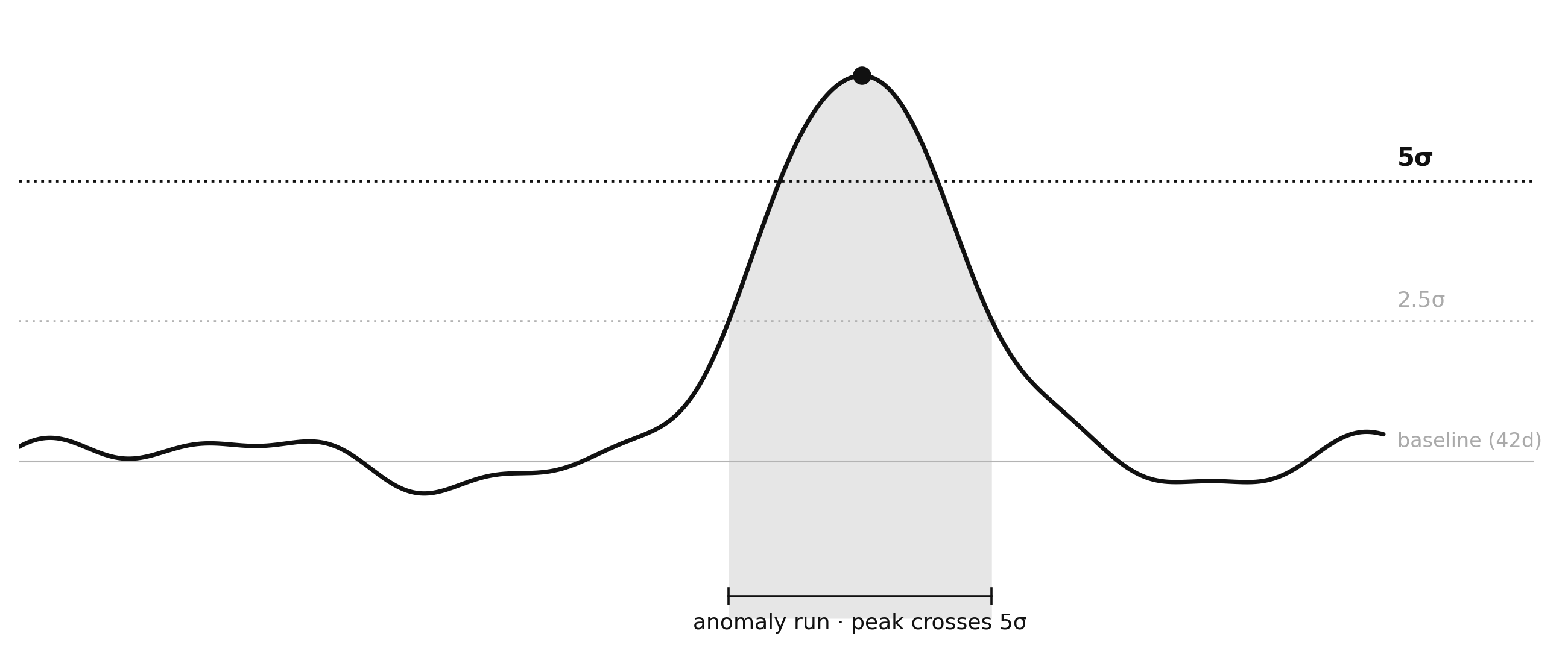
4. Dual-threshold interval detection. Rather than flagging every bucket above a single threshold, the algorithm uses two. A weak threshold (~2.5σ) defines a candidate run — a contiguous stretch of buckets above it. A strong threshold (default ~5σ) qualifies the run — at least one bucket somewhere inside it must cross 5σ for the run to count. This captures the rising and falling shoulders of a real spike, not just its peak.

We evaluated more elaborate formulations — forecasting models like ARIMA and Prophet, learned per-phrase detectors. The marginal lift over a well-tuned z-score did not justify the operational cost on real customer data. A good baseline can make simple detectors outperform sophisticated forecasters when the challenge is defining what’s “normal”. The complexity is better spent on building the baseline than on the detector.

Every threshold in the pipeline tunes the same tradeoff: false positives versus false negatives. Tighter thresholds keep noise out of the UI but suppress smaller real events. Looser thresholds catch more events but dilute the list. The current configuration favors recall — a missed outage costs more than a noisy candidate the downstream layers can filter — with per-customer knobs to tighten precision once we see what their data looks like.

Making Results Stable and Useful

A working detector is the first half of the product. The second half is making trends look like things you can act on rather than streams of phrases.

Phrase grouping. flight cancellation, cancelled flight, and flight cancel are the same trend. After statistical detection, an LLM-based clustering step groups equivalent phrases into a single trend object — and decides whether a newly spiking phrase is actually a re-emergence of an existing one. Singletons stay singletons; only multi-phrase groups merge. The shape of this — cluster equivalent phrases, then pick a single representative — is the same pattern Google Trends and Twitter Trending Now use to consolidate related items; the difference here is the input substrate (multi-turn conversations rather than search strings) and the use of an LLM for the grouping decision.

Noise filtering. Some phrases pass every statistical check and are still uninteresting — generic boilerplate, internal codes, transcription artifacts that happen to spike together. An LLM-based classifier marks top candidates as TREND or NOISE before they reach the UI. It fails open: if the classifier errors, the candidate goes through.

Trend lifecycle, not trend events. A spike that pops, fades, and pops again is one trend, not three. Each detection run reconciles new findings against the existing active set: continuing phrases extend their existing trend, stopped phrases transition the trend to inactive, and inactive trends can revive if their phrase re-spikes within a TTL window. The result is a small set of long-lived trend objects with full time-series history, not a firehose of independent events.

Human-readable names. A trend keyed on the literal phrase pluspoints expiring is technically correct but not glanceable in a dashboard. After detection, an LLM generates a short display name and one-line description per new trend, grounded in example messages. This runs once per trend on creation, not on every read.

Open a single trend and you get the named headline, its trajectory over time, and the conversations that drove it — enough to act on without leaving the page.

Email digests. New trends fan out as email digests with the generated headline and a snapshot chart, so responders see them without having to check the UI.

Lessons Learned

Here are a few initial observations from running this against real customer conversation streams.

Simple wins, but only with the right scaffolding around it. The detection core is classical statistics. The complexity budget went into baselines, smoothing, deduplication, state tracking, and naming. That is where the production quality came from — not from a fancier detector.

LLMs at the edges, not in the hot loop. Language models do the messy, infrequent, high-value work: naming, clustering, noise filtering. They never touch the per-bucket detection step, which keeps cost and latency predictable and makes failures easy to reason about.

Pick infrastructure that absorbs the boring work. ClickHouse handles rollups, deduplication, incoming/aggregated/cold retention, and partition expiry through built-in primitives — we never wrote a custom batch job for any of it. Rust and PyO3 handle the per-message extraction loop so the Python orchestration layer can stay focused on workflows. In both cases the saved complexity went straight into the algorithm.

Extraction sets the ceiling. What looked like setup details — tokenization, stopword choice, phrase canonicalization — drove more downstream signal quality than the detector itself. Decisions like keeping due and first as content words because they carry meaning in support contexts only emerged from running the system on real conversations.

Noisy language is the hardest part. Transcription errors split the same event across multiple phrases. Brand names tokenize inconsistently. Multilingual content stresses every layer. The system handles a large fraction of this through normalization and clustering, but it stays an active area of iteration.

Evaluation often has no ground truth. There is no labeled corpus of real trends. Offline metrics are weak proxies. The most reliable feedback signal comes from customers running the system over their own data — which is why we're rolling this out as a closed early-access program, structured around tight feedback loops with the first few customers rather than a blind general release.

The shape of the system reflects the shape of the problem. The per-bucket detection step is statistical — a z-score against a baseline, deterministic and cheap. Naming, clustering, and noise filtering are LLM-driven, but they fire only on newly detected trends — the narrow end of a funnel that started with millions of ngrams. Detecting black swans in conversation data turns out to be less about clever statistics than about getting the unglamorous infra parts — extraction, baselines, state management — exactly right.